
Data Dictionary
There are multiple variables in the dataset: divided in 3 categories:
Demographic information about customers
customer_id - Customer id
vintage - Vintage of the customer with the bank in number of days
age - Age of customer
gender - Gender of customer
dependents - Number of dependents
occupation - Occupation of the customer
city - City of customer (anonymised)
Customer Bank Relationship
customer_nw_category - Net worth of customer (3:Low 2:Medium 1:High)
branch_code - Branch Code for customer account
days_since_last_transaction - No of Days Since Last Credit in Last 1 year
Transactional Information
current_balance - Balance as of today
previous_month_end_balance - End of Month Balance of previous month
average_monthly_balance_prevQ - Average monthly balances (AMB) in Previous Quarter
average_monthly_balance_prevQ2 - Average monthly balances (AMB) in previous to previous quarter
current_month_credit - Total Credit Amount current month
previous_month_credit - Total Credit Amount previous month
current_month_debit - Total Debit Amount current month
previous_month_debit - Total Debit Amount previous month
current_month_balance - Average Balance of current month
previous_month_balance - Average Balance of previous month
churn - Average balance of customer falls below minimum balance in the next quarter (1/0)
Churn Prediction using Logisitic Regression
Now, that I understand the dataset in detail. It is time to build a logistic regression model to predict the churn. I have included the data dictionary above for reference.
Load Data & Packages for model building & preprocessing
Preprocessing & Missing value imputation
Select features on the basis of EDA Conclusions & build baseline model
Decide Evaluation Metric on the basis of business problem
Build model using all features & compare with baseline
Use Reverse Feature Elimination to find the top features and build model using the top 10 features & compare
Loading Packages
import numpy as np
import pandas as pd
import seaborn as sns
import matplotlib.pyplot as plt
from sklearn.preprocessing import LabelEncoder
from sklearn.preprocessing import StandardScaler
from sklearn.linear_model import LogisticRegression
from sklearn.model_selection import KFold, StratifiedKFold, train_test_split
from sklearn.metrics import roc_auc_score, accuracy_score, confusion_matrix, roc_curve, precision_score, recall_score, precision_recall_curve
import warnings
warnings.simplefilter(action='ignore', category=FutureWarning)
warnings.simplefilter(action='ignore', category=UserWarning)
Loading Data
df_churn = pd.read_csv('bank_customer_data.csv') |
Missing Values
Before I go on to build the model, I must look for missing values within the dataset as treating the missing values is a necessary step before I fit a logistic regression model on the dataset.
pd.isnull(df_churn).sum() customer_id 0
vintage 0
age 0
gender 525
dependents 2463
occupation 80
city 803
customer_nw_category 0
branch_code 0
days_since_last_transaction 3223
current_balance 0
previous_month_end_balance 0
average_monthly_balance_prevQ 0
average_monthly_balance_prevQ2 0
current_month_credit 0
previous_month_credit 0
current_month_debit 0
previous_month_debit 0
current_month_balance 0
previous_month_balance 0
churn 0
dtype: int64 |
The result of this function shows that there are quite a few missing values in columns gender, dependents, city, days since last transaction and Percentage change in credits. I go through each of them 1 by 1 to find the appropriate missing value imputation strategy for each of them.
Gender For a quick recall look at the categories within gender column
df_churn['gender'].value_counts() Male 16548
Female 11309
Name: gender, dtype: int64 |
So there is a good mix of males and females and arguably missing values cannot be filled with any one of them. I could create a seperate category by assigning the value -1 for all missing values in this column.
Before that, first I will convert the gender into 0/1 and then replace missing values with -1
#Convert Gender dict_gender = {'Male': 1, 'Female':0} df_churn.replace({'gender': dict_gender}, inplace = True) df_churn['gender'] = df_churn['gender'].fillna(-1) |
Dependents, occupation and city with mode
Next I will have a quick look at the dependents & occupations column and impute with mode as this is sort of an ordinal variable
df_churn['dependents'].value_counts() 0.0 21435
2.0 2150
1.0 1395
3.0 701
4.0 179
5.0 41
6.0 8
7.0 3
9.0 1
52.0 1
36.0 1
50.0 1
8.0 1
25.0 1
32.0 1
Name: dependents, dtype: int64 |
df_churn['occupation'].value_counts()
self_employed 17476
salaried 6704
student 2058
retired 2024
company 40
Name: occupation, dtype: int64
df_churn['dependents'] = df_churn['dependents'].fillna(0)
df_churn['occupation'] = df_churn['occupation'].fillna('self_employed')
Similarly City can also be imputed with most common category 1020
df_churn['city'] = df_churn['city'].fillna(1020) |
Days since Last Transaction
A fair assumption can be made on this column as this is number of days since last transaction in 1 year, I can substitute missing values with a value greater than 1 year say 999
df_churn['days_since_last_transaction'] = df_churn['days_since_last_transaction'].fillna(999) |
Preprocessing
Now, before applying linear model such as logistic regression, I need to scale the data and keep all features as numeric strictly.
Dummies with Multiple Categories
# Convert occupation to one hot encoded features df_churn = pd.concat([df_churn,pd.get_dummies(df_churn['occupation'],prefix = str('occupation'),prefix_sep='_')],axis = 1) |
Scaling Numerical Features for Logistic Regression
Now, I remember that there are a lot of outliers in the dataset especially when it comes to previous and current balance features. Also, the distributions are skewed for these features if you recall from the EDA. I will take 2 steps to deal with that here:
Log Transformation
Standard Scaler
Standard scaling is anyways a necessity when it comes to linear models and I have done that here after doing log transformation on all balance features.
num_cols = ['customer_nw_category', 'current_balance', 'previous_month_end_balance', 'average_monthly_balance_prevQ2', 'average_monthly_balance_prevQ', 'current_month_credit','previous_month_credit', 'current_month_debit', 'previous_month_debit','current_month_balance', 'previous_month_balance'] for i in num_cols: df_churn[i] = np.log(df_churn[i] + 17000) std = StandardScaler() scaled = std.fit_transform(df_churn[num_cols]) scaled = pd.DataFrame(scaled,columns=num_cols) |
df_df_og = df_churn.copy() df_churn = df_churn.drop(columns = num_cols,axis = 1) df_churn = df_churn.merge(scaled,left_index=True,right_index=True,how = "left") |
y_all = df_churn.churn df_churn = df_churn.drop(['churn','customer_id','occupation'],axis = 1) |
Model Building and Evaluation Metrics
Since this is a binary classification problem, I could use the following 2 popular metrics:
Recall
Area under the Receiver operating characteristic curve
Now, I am looking at the recall value here because a customer falsely marked as churn would not be as bad as a customer who was not detected as a churning customer and appropriate measures were not taken by the bank to stop him/her from churning The ROC AUC is the area under the curve when plotting the (normalized) true positive rate (x-axis) and the false positive rate (y-axis). My main metric here would be Recall values, while AUC ROC Score would take care of how well predicted probabilites are able to differentiate between the 2 classes.
Conclusions from Exploratory Data Analysis (EDA)
For debit values, I see that there is a significant difference in the distribution for churn and non churn and it might be turn out to be an important feature
For all the balance features the lower values have much higher proportion of churning customers
For most frequent vintage values, the churning customers are slightly higher, while for higher values of vintage, I have mostly non churning customers which is in sync with the age variable
I see significant difference for different occupations and certainly would be interesting to use as a feature for prediction of churn.
Now, I will first split my dataset into test and train and using the above conclusions select columns and build a baseline logistic regression model to check the ROC-AUC Score & the confusion matrix
Baseline Columns
baseline_cols = ['current_month_debit', 'previous_month_debit','current_balance','previous_month_end_balance','vintage' ,'occupation_retired', 'occupation_salaried','occupation_self_employed', 'occupation_student'] |
df_baseline = df_churn[baseline_cols] |
Train Test Split to create a validation set
# Splitting the data into Train and Validation set xtrain, xtest, ytrain, ytest = train_test_split(df_baseline,y_all,test_size=1/3, random_state=11, stratify = y_all) |
model = LogisticRegression() model.fit(xtrain,ytrain) pred = model.predict_proba(xtest)[:,1] |
AUC ROC Curve & Confusion Matrix
from sklearn.metrics import roc_curve fpr, tpr, _ = roc_curve(ytest,pred) auc = roc_auc_score(ytest, pred) plt.figure(figsize=(12,8)) plt.plot(fpr,tpr,label="Validation AUC-ROC="+str(auc)) x = np.linspace(0, 1, 1000) plt.plot(x, x, linestyle='-') plt.xlabel('False Positive Rate') plt.ylabel('True Positive Rate') plt.legend(loc=4) plt.show() |
 |
# Confusion Matrix pred_val = model.predict(xtest) |
label_preds = pred_val cm = confusion_matrix(ytest,label_preds) def plot_confusion_matrix(cm, normalized=True, cmap='bone'): plt.figure(figsize=[7, 6]) norm_cm = cm if normalized: norm_cm = cm.astype('float') / cm.sum(axis=1)[:, np.newaxis] sns.heatmap(norm_cm, annot=cm, fmt='g', xticklabels=['Predicted: No','Predicted: Yes'], yticklabels=['Actual: No','Actual: Yes'], cmap=cmap) plot_confusion_matrix(cm, ['No', 'Yes']) |
 |
# Recall Score recall_score(ytest,pred_val) |
0.11580148317170565 |
Cross validation
Cross Validation is one of the most important concepts in any type of data modelling. It simply says, try to leave a sample on which you do not train the model and test the model on this sample before finalizing the model.
I divide the entire population into k equal samples. Now I train models on k-1 samples and validate on 1 sample. Then, at the second iteration I train the model with a different sample held as validation.
In k iterations, I have basically built the model on each sample and held each of them as validation. This is a way to reduce the selection bias and reduce the variance in prediction power.
Since it builds several models on different subsets of the dataset, I can be more certain of model performance if I use CV for testing my models.
def cv_score(ml_model, rstate = 12, thres = 0.5, cols = df_churn.columns): i = 1 cv_scores = [] df1 = df_churn.copy() df1 = df_churn[cols]
# 5 Fold cross validation stratified on the basis of target kf = StratifiedKFold(n_splits=5,random_state=rstate,shuffle=True) for df_index,test_index in kf.split(df1,y_all): print('\n{} of kfold {}'.format(i,kf.n_splits)) xtr,xvl = df1.loc[df_index],df1.loc[test_index] ytr,yvl = y_all.loc[df_index],y_all.loc[test_index]
# Define model for fitting on the training set for each fold model = ml_model model.fit(xtr, ytr) pred_probs = model.predict_proba(xvl) pp = []
# Use threshold to define the classes based on probability values for j in pred_probs[:,1]: if j>thres: pp.append(1) else: pp.append(0)
# Calculate scores for each fold and print pred_val = pp roc_score = roc_auc_score(yvl,pred_probs[:,1]) recall = recall_score(yvl,pred_val) precision = precision_score(yvl,pred_val) sufix = "" msg = "" msg += "ROC AUC Score: {}, Recall Score: {:.4f}, Precision Score: {:.4f} ".format(roc_score, recall,precision) print("{}".format(msg))
# Save scores cv_scores.append(roc_score) i+=1 return cv_scores |
baseline_scores = cv_score(LogisticRegression(), cols = baseline_cols) |
1 of kfold 5 ROC AUC Score: 0.7644836090843695, Recall Score: 0.0751, Precision Score: 0.5766 2 of kfold 5 ROC AUC Score: 0.779451238310554, Recall Score: 0.0751, Precision Score: 0.6695 3 of kfold 5 ROC AUC Score: 0.7551621478942728, Recall Score: 0.1350, Precision Score: 0.6425 4 of kfold 5 ROC AUC Score: 0.7582070977015274, Recall Score: 0.1169, Precision Score: 0.6508 5 of kfold 5 ROC AUC Score: 0.7632311004249608, Recall Score: 0.1112, Precision Score: 0.5850 |
Now I will try using all columns available to check if I get significant improvement.
all_feat_scores = cv_score(LogisticRegression()) |
1 of kfold 5 ROC AUC Score: 0.7322735587298325, Recall Score: 0.1093, Precision Score: 0.5066 2 of kfold 5 ROC AUC Score: 0.7681477751515774, Recall Score: 0.1968, Precision Score: 0.6809 3 of kfold 5 ROC AUC Score: 0.7392333107476944, Recall Score: 0.1673, Precision Score: 0.5714 4 of kfold 5 ROC AUC Score: 0.7394851378820373, Recall Score: 0.1597, Precision Score: 0.6667 5 of kfold 5 ROC AUC Score: 0.758833273580065, Recall Score: 0.1730, Precision Score: 0.5987 |
There is some improvement in both ROC AUC Scores and Precision/Recall Scores. Now I can try backward selection to select the best subset of features which give the best score.
Reverse Feature Elimination or Backward Selection
I have already built a model using all the features and a separate model using some baseline features. I can try using backward feature elimination to check if I can do better. I will do that next.
from sklearn.feature_selection import RFE import matplotlib.pyplot as plt # Create the RFE object and rank each feature model = LogisticRegression() rfe = RFE(estimator=model, n_features_to_select=1, step=1) rfe.fit(df_churn, y_all) |
RFE(estimator=LogisticRegression(), n_features_to_select=1) |
ranking_df = pd.DataFrame() ranking_df['Feature_name'] = df_churn.columns ranking_df['Rank'] = rfe.ranking_ |
ranked = ranking_df.sort_values(by=['Rank']) |
ranked |
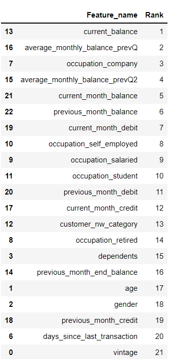
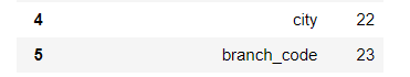
The balance features are proving to be very important as can be seen from the table. The RFE function can also be used to select features. I selected the top 10 features from this table and checked score.
rfe_top_10_scores = cv_score(LogisticRegression(), cols = ranked['Feature_name'][:10].values) |
1 of kfold 5 ROC AUC Score: 0.7986881101633954, Recall Score: 0.2281, Precision Score: 0.7362 2 of kfold 5 ROC AUC Score: 0.8050442914397288, Recall Score: 0.2234, Precision Score: 0.7556 3 of kfold 5 ROC AUC Score: 0.7985130070256687, Recall Score: 0.2205, Precision Score: 0.7250 4 of kfold 5 ROC AUC Score: 0.7935095616193245, Recall Score: 0.2120, Precision Score: 0.7360 5 of kfold 5 ROC AUC Score: 0.7942222838028076, Recall Score: 0.1911, Precision Score: 0.6745 |
Wow, the top 10 features obtained using the reverse feature selection are giving a much better score than any of our earlier attempts. This is the power of feature selection and it especially works well in case of linear models as tree based models are in itself to some extent capable of doing feature selection.
The recall score here is quite low. I should play around with the threshold to get a better recall score. AUC ROC depends on the predicted probabilities and is not impacted by the threshold. I will try 0.2 as threshold which is close to the overall churn rate
cv_score(LogisticRegression(), cols = ranked['Feature_name'][:10].values, thres=0.14) |
1 of kfold 5 ROC AUC Score: 0.7986881101633954, Recall Score: 0.8308, Precision Score: 0.2836 2 of kfold 5 ROC AUC Score: 0.8050442914397288, Recall Score: 0.8375, Precision Score: 0.2902 3 of kfold 5 ROC AUC Score: 0.7985130070256687, Recall Score: 0.8279, Precision Score: 0.2897 4 of kfold 5 ROC AUC Score: 0.7935095616193245, Recall Score: 0.8213, Precision Score: 0.2840 5 of kfold 5 ROC AUC Score: 0.7942222838028076, Recall Score: 0.8108, Precision Score: 0.2927 |
[0.7986881101633954, 0.8050442914397288, 0.7985130070256687, 0.7935095616193245, 0.7942222838028076] |
I observe that there is continuous improvement in the Recall Score. However, clearly precision score is going down. On the basis of business requirement the bank can take a call on deciding the threshold. Without knowing the metrics relevant to the business, the best course of action is to optimize for AUC ROC Score so as to find the best probabilities here.
コメント