
Building a classifier using Spotify API and KNN
Everyone loves music, and loves to listen to multiple artists. Each artist is unique and interesting. But how unique, and how interesting? In this project, I set out to create a machine learning model that would be able to predict who the artist is. I first listed my favorite artists, then used the Spotify API to get song data from their top 10 songs, cleaned and preprocessed that data, and then used the K-Nearest Neighbor algorithm to create a machine learning model to predict a song’s artist. My algorithm was ~50% accurate.
🎸Getting The Song Data
First, I needed to name the artists that I was most interested in. I could do every possible artist, but that would take a lot more work, so I chose to focus on the artists I am personally interested in. For me that was: Taylor Swift, Kanye West, John Mayer, The Beatles, Imagine Dragons, Ed Sheeran, Tim McGraw, Billie Elish, and AJR.
Next, I needed credentials for the Spotify API use. You can follow along on how to get those via this link here. I also needed to understand what endpoints were available in the API which took a little bit of research and playing. You can read endpoint docs here. Instead of using the actual API with HTTP Requests, I found a Python wrapper called Spotipy that made the data collection easier
The individual song data is available at the audio-features endpoint. But that requires the Spotify ID’s of the individual tracks. So I first needed to collect those. Those ID’s can be found in the track information that is given by artist-top-tracks endpoint. BUT that endpoint requires the Spotify Artist ID, which is not the artist name so I used Spotify API endpoint of search to search the artist’s name and pull their Artist ID.
After I had the Artist ID’s, I could then pull their top songs, and pull the data for each of those songs. Then the results were saved to a CSV file. See code below.
#Collect the songs into a DB #list artists of interest artists = ['Taylor Swift', 'John Mayer', 'Ed Sheeran', 'The Beatles', 'George Strait','The Judds', 'Tim McGraw','Billie Elish','AJR'] df_final = pd.DataFrame() for i in range(0,len(artists)): #for artists #finding artist ID artist = artists[i] results = sp.search(q='artist: ' + artist, type='artist') items = results['artists']['items'] id_i = items[0]['external_urls']['spotify'].split('/')[-1] ids.append(id_i) #finding top tracks top_tracks = sp.artist_top_tracks(id_i,country='US') track_info = top_tracks['tracks'] num_tracks = len(track_info) for j in range(0,num_tracks): song_id = track_info[j]['id'] song_name = track_info[j]['name'] song_features = sp.audio_features(song_id)[0] #add info song_features['song_name'] = song_name song_features['artist'] = artist row = pd.DataFrame(song_features, index=[0]) df_final = df_final.append(row) df_final = df_final[['song_name','artist','danceability', 'energy', 'key', 'loudness', 'mode', 'speechiness','acousticness', 'instrumentalness', 'liveness', 'valence', 'tempo','duration_ms']] df_final.to_csv('artists_database.csv') |
The resulting dataframe/CSV looked something like this:
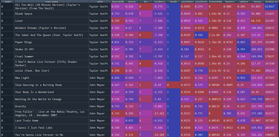
Spotify Data Table (Created by Author)
📊Exploratory Data Analysis
After creating the data set, the next step was to explore it. Using Seaborn’s pairplot function I was able to evaluate the relationship of all our our columns.
# Libraries import pandas as pd import seaborn as sns #Import data df = pd.read_csv('C://DataCareerJumpstart//artists_database.csv') #Pair plot sns.pairplot(df.drop(['Unnamed: 0','mode','song_name'],axis=1), hue='artist') #Correlation |
💻Preprocessing The Data
I knew I wanted to do classification, and chose K-Nearest Neighbor as the first model to test out. As always with supervised learning, I split my data into training data sets, selecting 70% for training and 30% for testing.
x_cols = ['danceability','energy','key','loudness','mode', 'speechiness','acousticness','instrumentalness', 'liveness','valence','tempo','duration_ms'] #splitting to testing /training from sklearn.model_selection import train_test_split X_train, X_test, y_train, y_test = train_test_split(df[x_cols],df['artist'],train_size=.7,random_state=0) |
To get the best result, I wanted to mean-center and scale my data. I did this pretty simply with sklearn.
from sklearn.preprocessing import StandardScaler #Takes off the song name (last column) X_train_data = X_train.iloc[:,:-1].reset_index(drop=True) X_test_data = X_test.iloc[:,:-1].reset_index(drop=True) # transform data scalar = StandardScaler() X_train_data = scalar.fit_transform(X_train_data) X_test_data = scalar.fit_transform(X_test_data) |
🤖Creating ML Model
K-Nearest Neighbors is a great classification algorithm that uses distances to compute the majority neighbor and votes the unknown sample as the majority neighbor’s class or group.
In this case, I was using the features of the song (‘danceability’, ‘energy’, ‘key’, ‘loudness’, ‘mode’, ‘speechiness’, ‘acousticness’, ‘instrumentalness’, ‘liveness’, ‘valence’, ‘tempo’, ‘duration’) to predict the artist’s name.
I selected k=6, just as a guess, and one can always adjust k to see if the accuracy increases. The algorithm is easy to create using scikit learn:
#Classification from sklearn.neighbors import KNeighborsClassifier #Make the KNN model knn = KNeighborsClassifier(n_neighbors=6) knn.fit(X_train_data, y_train) #Train the data predictions = knn.predict(X_train_data) # Making predictions on training data print(knn.score(X_train_data,y_train)) # give the accuracy |
The accuracy for this model on the training day was 48%.
👀Visualizing & Evaluating The Model
Not only did I want to see the accuracy, but also understand how the model was working so I created two ways to visualize the model: a confusion matrix and a decision surface plot.
A confusion matrix allows one to understand how the model classifies on different class labels and gives more insight into what labels are easier or harder to predict.
Once again, making the confusion matrix was pretty easy in scikit learn with only a few lines of code:
#Confusion matrix for training data comparisons = pd.DataFrame() predictions = predictions actuals = y_train.to_list() song_name = X_train.iloc[:,-1].to_list() #Visually understand that now from sklearn.metrics import confusion_matrix, ConfusionMatrixDisplay import matplotlib.pyplot as plt cm = confusion_matrix(y_train, predictions, labels=knn.classes_) disp = ConfusionMatrixDisplay(confusion_matrix=cm, display_labels=knn.classes_) disp.plot() plt.tick_params(axis="x", labelrotation=90) plt.title('Confusion Matrix (Training) ') plt.show() |
The resulting plot helped me understand the model more:

Confusion Matrix For Training (Image by Author)
We also tested the accuracy and confusion matrix of the testing data. The accuracy dropped to 33% and here is the resulting confusion matrix:

Confusion Matrix For Testing (Image by Author)
And of course, the decision surface was created using the following snippet:
import numpy as np h = .02 #step size in the mesh # create a mesh to plot in x_min, x_max = X_train.iloc[:, 0].min() - .2, X_train.iloc[:, 0].max() + .2 y_min, y_max = X_train.iloc[:, 1].min() - .2, X_train.iloc[:, 1].max() + .2 xx, yy = np.meshgrid(np.arange(x_min, x_max, h), np.arange(y_min, y_max, h)) knn2 = KNeighborsClassifier(n_neighbors=6) knn2.fit(X_train_data[:,:2], y_train.astype("category").cat.codes) Z = knn2.predict(np.c_[xx.ravel(), yy.ravel()]) #Put the result into a color plot Z = Z.reshape(xx.shape) plt.figure() plt.contour(xx, yy, Z, cmap=plt.cm.Pastel1, alpha=0.8) # Plot the training points also plt.scatter(X_train.iloc[:, 0], X_train.iloc[:, 1], c = y_train.astype("category").cat.codes, cmap=plt.cm.Pastel1, edgecolors='k') plt.xlabel('dancibility') plt.ylabel('energy') plt.xlim(xx.min(), xx.max()) plt.ylim(yy.min(), yy.max()) plt.xticks(()) plt.yticks(()) plt.show() |
And resulted in this image:
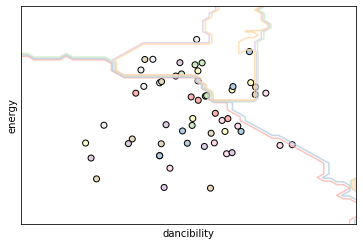
Decision Surface for Dancibility and Energy
To improve the decision surface plot, I decided to use PCA to lower dimensions to make the visualization a little bit more interesting. Here’s the code I used to perform the PCA:
# Now let's try PCA from sklearn import decomposition pca = decomposition.PCA(n_components=5) pca.fit(X_train_data) X_train_pca = pca.transform(X_train_data) print('Variable explanations: ') print(pca.explained_variance_ratio_) |
PC1 and PC2 accounted for 28% and 13% of the variance respectively. And the new graph told a little bit more of an understandable story:

Decision Surface for PC1 and PC2
# Plot in PCA# create a mesh to plot in x_min, x_max = X_train_pca[:, 0].min() - .2, X_train_pca[:, 0].max() + .2 y_min, y_max = X_train_pca[:, 1].min() - .2, X_train_pca[:, 1].max() + .2 xx, yy = np.meshgrid(np.arange(x_min, x_max, h), np.arange(y_min, y_max, h)) knn2 = KNeighborsClassifier(n_neighbors=3) knn2.fit(X_train_pca[:,:2], y_train.astype("category").cat.codes) print('PCA Training Accuracy:') print(knn2.score(X_train_pca[:,:2], y_train.astype("category").cat.codes)) Z = knn2.predict(np.c_[xx.ravel(), yy.ravel()]) # Put the result into a color plot Z = Z.reshape(xx.shape) plt.figure() plt.contourf(xx, yy, Z, cmap=plt.cm.Pastel1, alpha=0.8) # Plot also the training points plt.scatter(X_train_pca[:, 0], X_train_pca[:, 1], c= y_train.astype("category").cat.codes, cmap=plt.cm.Pastel1, edgecolors ='k') plt.xlabel('PC1') plt.ylabel('PC2') plt.xlim(xx.min(), xx.max()) plt.ylim(yy.min(), yy.max()) plt.xticks(()) plt.yticks(()) plt.title('Decision Surface with PCA') plt.show() |
😎Model Made
Overall, I was able to create a pretty neat, unique machine learning algorithm that could somewhat classify an unknown song as the correct artist.
There is lots of room for improvement. For instance, I could be a bit more conscious of how I split the data as it was done randomly, but if for some reason there was an artist who was not selected in the training set, I could never predict them. I could have also collected more songs, and more artists to make the algorithm deeper and more robust.
Hope you enjoyed and let me know if you have any questions
Comments